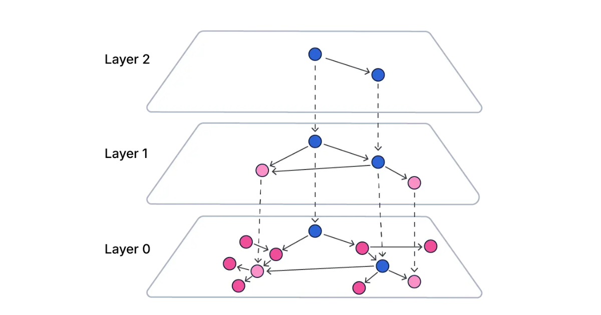
Similarity search in Chroma DB is generally straightforward, but there are a few important nuances to understand in order to use it effectively for information retrieval. Before exploring those details, it's helpful to first understand what a vector index is.

What is a Vector Index?

Finding the most semantically similar vectors to a query is mathematically straightforward. For example, to compute cosine similarity, you normalize the embeddings of all documents and the query, then calculate the dot product between the query embedding and each document embedding. This yields the cosine similarity scores. Identifying the most similar document is simply a matter of finding the one with the highest score.

However, this brute-force approach is inefficient—it requires comparing the query against every vector in the database, which becomes slow at scale. To address this, vector indexes are used. These are specialized data structures that enable algorithms to compute similarity scores with only a small subset of vectors, significantly speeding up the search while still returning exact or near-optimal results.

A vector index is specifically designed to store and organize high-dimensional embeddings for fast similarity and nearest neighbor searches. This organization is what enables vector indexes to scale to millions or even billions of vectors while maintaining low-latency performance. Instead of treating the dataset as a flat list, the index structures the data in a way that reflects the geometry of the vector space—clustering similar vectors together or linking them through proximity-based graphs. This allows the search algorithm to prune large portions of the dataset early in the search process, focusing only on the most promising regions.

What is a Hierarchical Navigable Small World (HNSW)?

HNSW is a fast, scalable graph-based vector index designed for approximate nearest neighbor (ANN) search in high-dimensional spaces. It is the sole indexing method supported by Chroma DB and is widely adopted in other vector databases due to its performance and reliability.

How It Works

HNSW builds a multi-layered graph where:

• The upper layers contain a sparse overview of the data for fast navigation.

• The bottom layer holds all vectors for detailed search.

Each vector connects to a few nearby neighbors, forming a "small world" network—meaning most vectors can be reached in just a few steps.

Search Process

The algorithm starts at the top layer and moves closer to the query vector as it descends, refining the search at each level. This structure allows it to skip most of the dataset and still find highly similar vectors quickly.

Why Use HNSW?

• Fast: Avoids scanning the entire dataset.

• Accurate: Delivers near-exact results.

• Scalable: Handles millions to billions of vectors.

• Versatile: Works with various similarity metrics.

Setting Up HNSW in Chroma DB

In Chroma DB, the HNSW vector index is configured during collection creation. Since HNSW is an approximate nearest neighbor algorithm, it's important to understand how its configuration affects both accuracy and performance. Parameters such as search speed, memory usage, and recall can all be tuned through the index settings. The example below demonstrates how to configure HNSW using the hnsw key:

    # setup
    import chromadb
    from chromadb.utils import embedding_functions
    ef = embedding_functions.SentenceTransformerEmbeddingFunction(
      model_name="all-MiniLM-L6-v2"
      )

    # Collection creation
    client = chromadb.Client()
    collection = client.create_collection(
      name="my_collection_name",
      metadata={"topic": "query testing"},
      configuration={
        "hnsw": {
          "space": "cosine",
          "ef_search": 100,
          "ef_construction": 100,
          "max_neighbors": 16
        },
        "embedding_function": ef
      }
    )

The key configuration parameters are:

• space: selects the distance metric. Possible options include:

  • l2: squared L2 (Euclidean) distance (default)

  • ip: inner (dot) product distance

  • cosine: cosine distance

• ef_search: the size of the candidate list used to search for nearest neighbors when a nearest neighbor search is performed. The default value is 100. Higher values improve both accuracy and recall, but at the cost of slower performance and increased computatuonal cost.

• ef_construction: the size of the candidate list used to select neighbors when a node is inserted during index construction. The default value is 100. Higher values improve the quality of the index and accuracy, but at the cost of slower performance and increased memory usage.

• max_neighbors: the maximum number of connections each node can have during construction. The defualt value is 16. Higher values lead to denser graphs that perform better during searches at the cost of higher memory usage and construction time.

We can categorize the performance-based parameters into two types:

• ef_search directly controls the breadth of the search at query time, making it the most direct lever for search quality (recall) vs. query speed.

• ef_construction and max_neighbors affect the quality of the built index. A higher-quality, denser index (achieved with higher ef_construction and max_neighbors provides a better foundation for searches, potentially leading to better accuracy. However, this quality comes at the cost of significantly longer index build times and higher memory consumption during construction and for storing the index.

Performing Similarity Searches in Chroma DB

# Add Data
collection.add(
    documents=[
        "Giant pandas are a bear species that lives in mountainous areas.",
        "A pandas DataFrame stores two-dimensional, tabular data",
        "I think everyone agrees that pandas are some of the cutest animals on the planet",
        "A direct comparison between pandas and polars indicates that polars is a more efficient library than pandas.",
    ],
    metadatas=[
        {"topic": "animals"},
        {"topic": "data analysis"},
        {"topic": "animals"},
        {"topic": "data analysis"},
    ],
    ids=["id1", "id2", "id3", "id4"]
)

# Querying in Chroma DB
collection.query(
    query_texts=["cats"],
    n_results=10,
)

'''
Note that querying the database involves passing the query, in a list, to the query_texts parameter in the .query() method. The optional parameter n_results controls the number of results to retrieve. In this case, n_results was set to 10, which exceeds the number of documents in the collection. Consequently, in this case, all results will be retrieved, ranked from most similar to the query to the least similar. The following presents the output of the above query:
'''

{'ids': [['id3', 'id1', 'id2', 'id4']],
 'embeddings': None,
 'documents': [['I think everyone agrees that pandas are some of the cutest animals on the planet',
   'Giant pandas are a bear species that lives in mountainous areas.',
   'A pandas DataFrame stores two-dimensional, tabular data',
   'A direct comparison between pandas and polars indicates that polars is a more efficient library than pandas.']],
 'uris': None,
 'included': ['metadatas', 'documents', 'distances'],
 'data': None,
 'metadatas': [[{'topic': 'animals'},
   {'topic': 'animals'},
   {'topic': 'data analysis'},
   {'topic': 'data analysis'}]],
 'distances': [[0.7380143404006958,
   0.8351750373840332,
   0.8634340167045593,
   0.9299634695053101]]}

# Querying with filters

collection.query(
    query_texts=["polar bear"],
    n_results=1,
)

{'ids': [['id4']],
 'embeddings': None,
 'documents': [['A direct comparison between pandas and polars indicates that polars is a more efficient library than pandas.']],
 'uris': None,
 'included': ['metadatas', 'documents', 'distances'],
 'data': None,
 'metadatas': [[{'topic': 'data analysis'}]],
 'distances': [[0.6243703365325928]]}

'''
What went wrong?
In this case, the word polar in the query was mistakenly matched with the term polars, referring to the Python data processing library mentioned in the document. As a result, the semantic search failed to retrieve documents about polar bears.

There are several ways to address this issue. One option is to refine the query by adding more context. Another is to try a different embedding model that may better capture the intended meaning. However, a simpler and more effective solution might be to apply filters to narrow the search results to a subset of the documents.

Consider the following code that enhances our original query by adding a metadata filter that narrows the search to documents about a specific topic:
'''

collection.query(
    query_texts=["polar bear"],
    n_results=1,
    where={'topic': 'animals'}
)

'''
The updated query now returns the correct result—a document about bears, rather than one related to Python libraries:
'''

'ids': [['id1']],
 'embeddings': None,
 'documents': [['Giant pandas are a bear species that lives in mountainous areas.']],
 'uris': None,
 'included': ['metadatas', 'documents', 'distances'],
 'data': None,
 'metadatas': [[{'topic': 'animals'}]],
 'distances': [[0.7096824645996094]]}

'''
Alternatively, instead of using a metadata filter, we could perform a full-text search to include or exclude documents based on specific words or phrases. For example, the following query excludes all documents that contain the word "library":
'''

collection.query(
    query_texts=["polar bear"],
    n_results=1,
    where_document={'$not_contains': 'library'}
)

collection.query(
    query_texts=["polar bear"],
    n_results=1,
    where={'topic': 'animals'},
    where_document={'$not_contains': 'library'}
)

Conclusion

In this reading, you gained a foundational understanding of how similarity search works in Chroma DB, with a focus on vector indexes and the Hierarchical Navigable Small World (HNSW) algorithm. Key topics covered include:

• Vector indexes fundamentals – how they structure high-dimensional data to enable efficient similarity searches.

• The HNSW algorithm – its use of a multi-layered graph to perform fast, scalable approximate nearest neighbor (ANN) searches.

• Configuring HNSW in Chroma DB – including key parameters like ef_search, ef_construction, and max_neighbors, and how they affect performance and accuracy.

• Executing similarity searches – from adding documents and querying semantically to interpreting results in context.

• Refining search results – using metadata filters and full-text constraints to enhance relevance and reduce semantic mismatches.